Multi-Dimensional CESE

CESE Dual Mesh

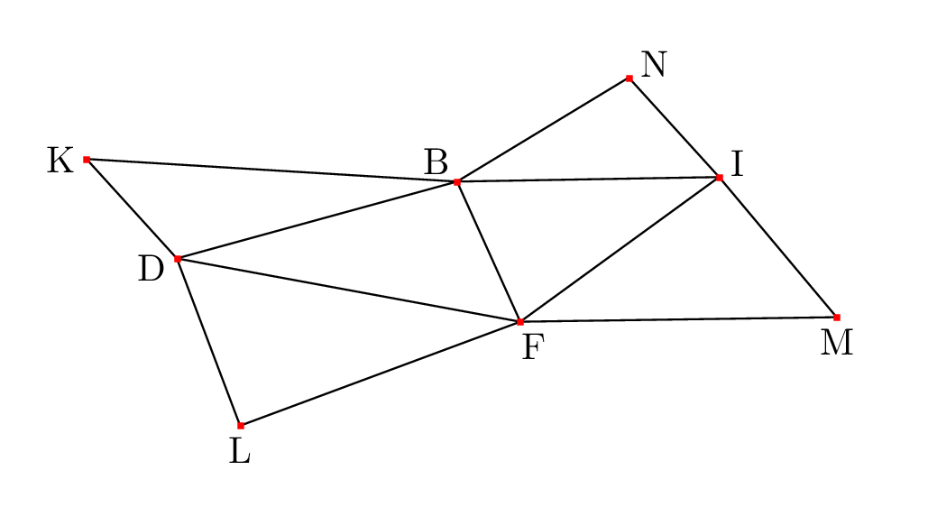
Fig. 12 Triangular mesh in two-dimensional space.

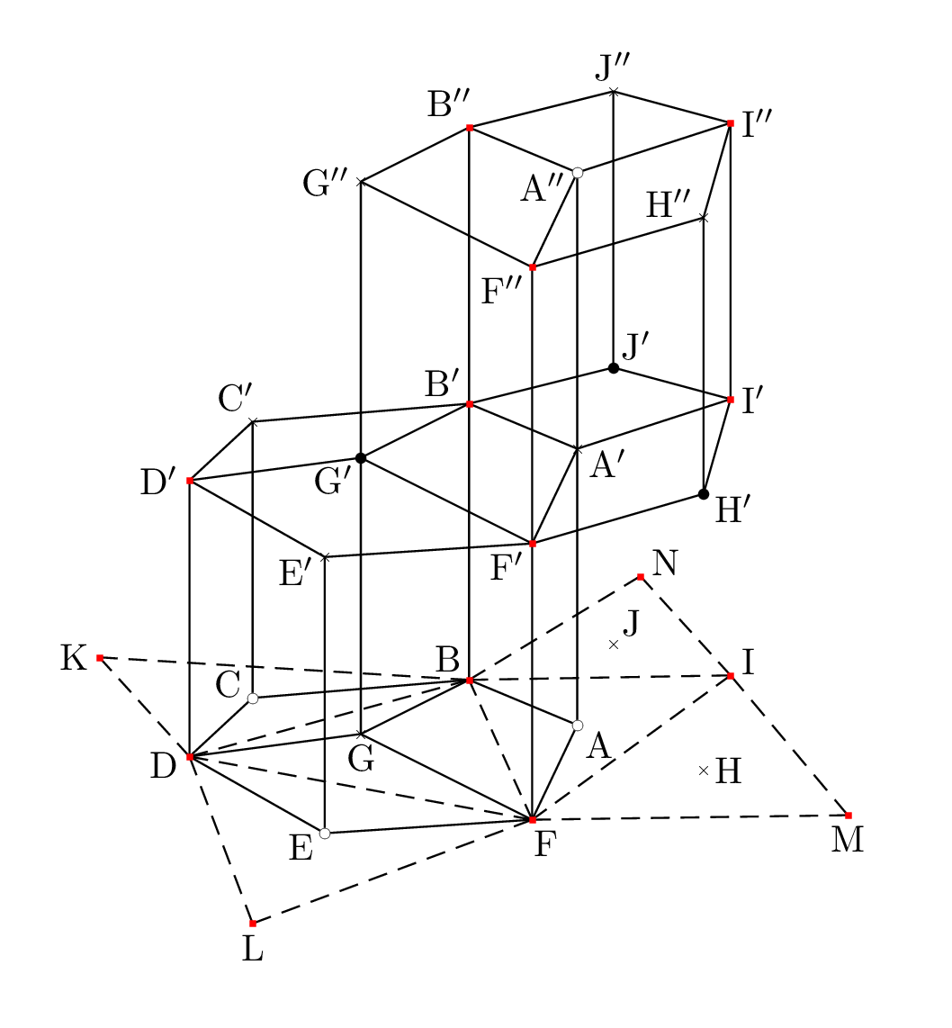
Fig. 13 Conservation elements of triangular meshes.

The figures above exhibit 6 triangles as an example of mesh elements for the CESE method. The CESE method evaluates the solutions at the centroids of conservation elements (CEs). The centroids are the solution points and are used to construct the solution elements (SEs). The element centers and the mesh vertices consist of the conservation elements. The conservation element is the space-time dual mesh defined on the unstructured mesh for the CESE method.

Gradient Elements

The CESE method \(c\)-scheme composes of evaluations of conservation and gradients. The first part assumes the gradients of the previous half time step as known to calculate the primary variables. The second part calculates the first-order derivative. To calculate the first-order derivative, we define gradient elements (GEs) [Che11]. There are two types of GEs: fundamental GE (FGE) and generalized GE (GGE). A FGE is a simplex in \(\mathbb{E}^N\) space. It always has \(N+1\) vertices. A GGE is a convex element composed of multiple non-overlapping FGEs that are separated by the GGE centroid.

In a FGE, the gradient of a scalar function \(\phi(\mathbf{x})\) is assumed to be constant, and denoted by

(7)\[\mathbf{g} \defeq \nabla\phi\]

Let \(\mathbf{x}^{(i)}\), \(i = 0, 1, \ldots, N\) be the coordinates of the vertices of a FGE. The coordinates define \(N\) displacement vectors

(8)\[\mathbf{d}^{(i)} \defeq \mathbf{x}^{(i)} - \mathbf{x}^{(0)}, \quad i = 1, \ldots, N\]

Combine all the displacement vectors to write the displacement matrix

(9)\[\begin{split}D \defeq \left(\begin{array}{ccc} d^{(1)}_1 & \cdots & d^{(1)}_N \\ \vdots & \ddots & \vdots \\ d^{(N)}_1 & \cdots & d^{(N)}_N \end{array}\right)\end{split}\]

Define

(10)\[\begin{split}\mathbf{q} \defeq \left(\begin{array}{c} \phi(\mathbf{x}^{(1)}) - \phi(\mathbf{x}^{(0)}) \\ \vdots \\ \phi(\mathbf{x}^{(N)}) - \phi(\mathbf{x}^{(0)}) \end{array}\right)\end{split}\]

and call it the difference vector. The system equation \(\mathbf{q} = \mathrm{D}\mathbf{g}\) can be written. \(\mathbf{q}\) and \(\mathrm{D}\) are known and \(\mathbf{g}\) is unknown. Write

(11)\[\mathbf{g} = \mathrm{D}^{-1}\mathbf{q}\]

The gradient \(\mathbf{g}\) defined in Eq. (7) is determined by Eqs. (8), (9), (10), and (11).

The gradient of a GGE is approximated by the average gradient at its centroid

(12)\[\mathbf{g}^c \defeq \frac{1}{M} \sum_{i=0}^{M-1} \mathbf{g}^{(i)}\]

where \(\mathbf{g}^{(0)}, \mathbf{g}^{(1)}, \ldots, \mathbf{g}^{(M-1)}\) are the gradient of its FGEs. If the GGE is a simplex, i.e., \(M = N+1\), it can be shown that \(\mathbf{g}^c\) is equal to the gradient calculated by treating the GGE as a FGE and applying Eq. (11).

W-1 Weighting Scheme

Eq. (12) leads to more interesting weighting functions for approximating GGE gradient for treating discontinuity. The W-1 scheme uses

\[ \mathbf{g}^{c} \approx \dfrac{ \sum\limits_{i=0}^{M-1} \left(\rho^{(i)}\right)^{\alpha}\mathbf{g}^{(i)} }{ \sum\limits_{i=0}^{M-1} \left(\rho^{(i)}\right)^{\alpha} } \]

where the weighting coefficients

\[ \rho^{(i)} \defeq \prod_{k=0; k\neq i}^{M-1} \left\vert\mathbf{g}^{(k)}\right\vert, \quad i = 0, \ldots, M-1 \]

and \(\alpha\) an adjustable parameter, usually a natural number.