Unstructured Meshes

We discretize the spatial domain of interest before solving PDEs. The discretized space is called a mesh [Mavriplis97]. When discretization is done by exploiting regularity in space, like cutting along each of the Cartesian coordinate axes, the discretized space is called a structured mesh. If the discretization does not follow any spatial order, we call the spatial domain an unstructured mesh. Both meshing strategies have their strength and weakness. Sometimes a structured mesh is also call a grid. Numerical methods that rely on spatial discretization are called mesh-based or grid-based.

To accommodate complex geometry, SOLVCON chose to use unstructured meshes of mixed elements. Because no structure is assumed for the geometry to be modeled, the mesh can be automatically generated by using computer programs. For example, the following image shows a triangular mesh of a two-dimensional irregular domain:

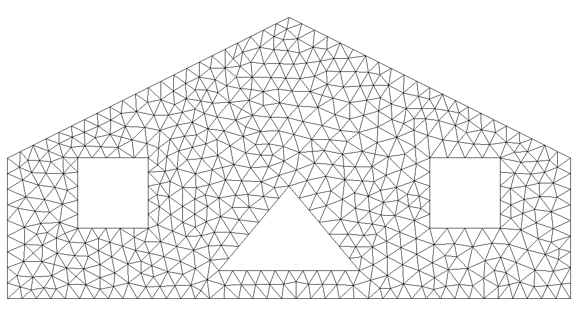
Figure 1: Two-dimensional sample mesh

which is generated by using the Gmsh (see the command file ustmesh_2d_sample.geo [1]). On the other hand, creation of structured meshes often needs a large amount of manual operations and will not be discussed in this document.

In SOLVCON, we assume a mesh is fully covered by a finite number of non-overlapping sub-regions, and only composed by these sub-regions. The sub-regions are called mesh elements. In one-dimensional space, SOLVCON also defines one type of mesh elements, line, as shown in Figure One-dimensional mesh element.

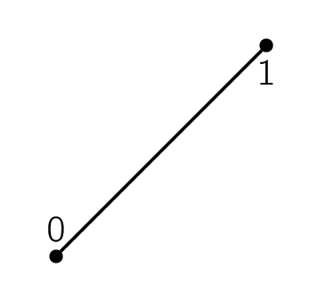
Figure 2: One-dimensional mesh element

SOLVCON allows two types of two-dimensional mesh elements, quadrilaterals and triangles, as shown in Figure Two-dimensional mesh elements, and four types of three-dimensional mesh elements, hexahedra, tetrahedra, prisms, and pyramids, as shown in Figure Three-dimensional mesh elements.

Figure 3: Two-dimensional mesh elements

Figure 4: Three-dimensional mesh elements

The numbers annotated in the figures are the order of the vertices of the elements. A SOLVCON mesh can be a mixture of elements of the same dimension, although it often only one element type.

Entities

Before explaining the data structure of the meshes, we need to introduce some basic terminologies and definitions. In SOLVCON, a cell means a mesh element. The dimensionality of a cell equals to that of the mesh it belongs to, e.g., a two-dimensional mesh is composed by two-dimensional cells. A cell is assumed to be concave, and enclosed by a set of faces. The dimensionality of a face is one less than that of a cell. A face is also assumed to be concave, and formed by connecting a sequence of nodes. The dimensionality of a node is at least one less than that of a face. Cells, faces, and nodes are the basic constructs, which we call entities, of a SOLVCON mesh.

Defining the term “entity” for SOLVCON facilitates a unified treatment of two- and three-dimensional meshes and the corresponding solvers [2]. A cell can be either two- or three-dimensional, and the associated faces become one- or two-dimensional, respectively. Because a face is either one- or two-dimensional, it can always be formed by a sequence of points, which is zero-dimensional. In this treatment, a point is equivalent to a node defined in the previous passage.

Take the two-dimensional mesh shown above as an example, triangular elements are used as the cells. The triangles are formed by three lines (one-dimensional shapes), which are the faces. Each line has two points (zero-dimensional). If we have a three-dimensional mesh composed by hexahedral cells, then the faces should be quadrilaterals (two-dimensional shapes).

All the mesh elements supported by SOLVCON are listed in the following table. The first column is the name of the element, and the second column is the type ID used in SOLVCON. The third column lists the dimensionality. The fourth, fifth, and sixth columns show the number of zero-, one-, and two-dimensional sub-entities belong to the element type, respectively. Note that the terms “point” and “line” appear in both the first row and first column, for they are the only element type in the space of the corresponding dimensionality.

Name	Type	Dim	Point#	Line#	Surface#
Point	0	0	0	0	0
Line	1	1	2	0	0
Quadrilateral	2	2	4	4	0
Triangle	3	2	3	3	0
Hexahedron	4	3	8	12	6
Tetrahedron	5	3	4	4	4
Prism	6	3	6	9	5
Pyramid	7	3	5	8	5

Although SOLVCON doesn’t support one-dimensional solvers, for completeness, we define the relation between one-dimensional cells (lines) and their sub-entities as:

Shape (type)	Face	= Point
Line (0)	0	\(\cdot\) 0
	1	\(\cdot\) 1

That is, as shown in Figure One-dimensional mesh element, a one-dimensional “cell” (line) has two “faces”, which are essentially point 0 and point 1. Symbol \(\cdot\) indicates a point.

It will be more practical to illustrate the relation between two-dimensional cells and their sub-entities in a table (see Figure Two-dimensional mesh elements for point locations):

Shape (type)	Face	= Line formed by points
Quadrilateral (2)	0	\(\diagup\) 0 1
	1	\(\diagup\) 1 2
	2	\(\diagup\) 2 3
	3	\(\diagup\) 3 0
Triangle (3)	0	\(\diagup\) 0 1
	1	\(\diagup\) 1 2
	2	\(\diagup\) 2 0

Symbol \(\diagup\) indicates a line. The orientation of lines of each two-dimensional shape is defined to follow the right-hand rule. The shape enclosed by the lines has an area normal vector points to the direction of \(+z\) (outward paper/screen).

The relation between three-dimensional cells and their sub-entities is defined in the table (see Figure Three-dimensional mesh elements for point locations):

Shape (type)	Face	= Surface formed by points
Hexahedron (4)	0	\(\square\) 0 3 2 1
	1	\(\square\) 1 2 6 5
	2	\(\square\) 4 5 6 7
	3	\(\square\) 0 4 7 3
	4	\(\square\) 0 1 5 4
	5	\(\square\) 2 3 7 6
Tetrahedron (5)	0	\(\triangle\) 0 2 1
	1	\(\triangle\) 0 1 3
	2	\(\triangle\) 0 3 2
	3	\(\triangle\) 1 2 3
Prism (6)	0	\(\triangle\) 0 1 2
	1	\(\triangle\) 3 5 4
	2	\(\square\) 0 3 4 1
	3	\(\square\) 0 2 5 3
	4	\(\square\) 1 4 5 2
Pyramid (7)	0	\(\triangle\) 0 4 3
	1	\(\triangle\) 1 4 0
	2	\(\triangle\) 2 4 1
	3	\(\triangle\) 3 4 2
	4	\(\square\) 0 3 2 1

Symbol \(\square\) indicates a quadrilateral, while symbol \(\triangle\) indicates a triangle.

Because a face is associated to two adjacent cells unless it’s a boundary face, it needs to identify to which cell it belongs, and to which cell it is neighbor. The area normal vector of a face is always point from the belonging cell to neighboring cell. The same rule applies to faces of two-dimensional meshes (lines) too.

Mesh Loading

A mesh is usually built up by using a mesh generator, like Gmsh. We then feed the generated mesh file to SOLVCON, which converts the unstructured-mesh data to the internal representation format: the Block class.

There are three steps required to fully construct a Block object: (i) instantiation, (ii) definition, and (iii) build-up. First, when instantiating an object, shape information must be provided to the constructor to allocate arrays for look-up tables:

from solvcon import Block
blk = Block(ndim=2, nnode=4, ncell=3)

Second, we fill the cell definition. Node coordinates and the node lists of cells need to be provided:

# Node coordinates.
blk.ndcrd[:,:] = (0,0), (-1,-1), (1,-1), (0,1)
# Cell types.
blk.cltpn[:] = 3
# Node list of cells.
blk.clnds[:,:4] = (3, 0,1,2), (3, 0,2,3), (3, 0,3,1)

Third, build up the rest of the object by calling (they will be explained later):

blk.build_interior()
blk.build_boundary()
blk.build_ghost()

Block.build_interior()

Building up a Block object includes two steps. First, the method deduce information from the defined arrays cltpn and clnds to create the arrays clfcs, fctpn, fcnds, and fccls. If the number of extracted faces is not the same as that passed into the constructor, arrays related to faces are recreated.

The method then fills all the geometry arrays from Block.ndcrd.

Block.build_boundary()

This method iterates over each of the BC objects listed in Block.bclist to collect boundary-condition information and build boundary faces. If a face belongs to only one cell (i.e., has no neighboring cell), it is regarded as a boundary face.

Unspecified boundary faces will be collected to form an additional BC object. It sets bndfcs for later use by build_ghost().

Block.build_ghost()

This method creates the shared arrays, calculates the information for ghost cells, and reassigns interior arrays as the right portions of the shared arrays. Only after this ghost build-up process, the Block object can be used by solvers.

Block.bndfcs

Type:numpy.ndarray

The array is of shape (nbound, 2) and type int32. Each row contains the data for a boundary face. The first column is the 0-based index of the face, while the second column is the serial number of the associated solvcon.boundcond.BC object.

We then can save the block to a VTK file for viewing:

from solvcon.io.vtkxml import VtkXmlUstGridWriter
iodev = VtkXmlUstGridWriter(blk)
iodev.write('block_2d_sample.vtu')

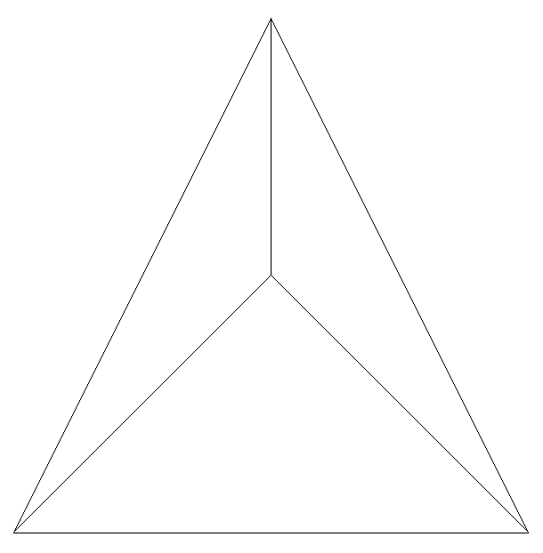
Figure 5: A simple Block object

class solvcon.Block(ndim=0, nnode=0, nface=0, ncell=0, nbound=0, use_incenter=False)

This class represents the unstructured meshes used in SOLVCON. As such, in SOLVCON, an unstructured mesh is also called a “block”. The following six attributes can be passed into the constructor. ndim, nnode, and ncell need to be non-zero to instantiate a valid block. nface and nbound might be different to the given value after building up the object. use_incenter is an optional flag.

ndim

Type:int

Number of dimensionalities of this mesh. Read only after instantiation.

nnode

Type:int

Total number of (non-ghost) nodes of this mesh. Read only after instantiation.

nface

Type:int

Total number of (non-ghost) faces of this mesh. Read only after instantiation.

ncell

Type:int

Total number of (non-ghost) cells of this mesh. Read only after instantiation.

nbound

Type:int

Total number of boundary faces or ghost cells of this mesh. Read only after instantiation.

use_incenter

Type:bool

Indicates calculating incenters instead of centroids for cells. Default is False (using centroids of cells).

The meshes are defined by three sets of look-up tables (arrays): (i) geometry, (ii) type, and (iii) connectivity.

Geometry Tables

ndcrd

Coordinates of nodes. It’s a two-dimensional numpy.ndarray array of shape (nnode, ndim) of type float64.

fccnd

Centroids of faces. It’s a two-dimension numpy.ndarray of shape (nface, ndim) of type float64.

fcnml

Unit normal vectors of faces. It’s a two-dimension numpy.ndarray of shape (nface, ndim) of type float64.

fcara

Areas of faces. The value should always be non-negative. It’s a one-dimension numpy.ndarray of shape (nface,) of type float64.

clcnd

Centroids of cells. It’s a two-dimension numpy.ndarray of shape (ncell, ndim) of type float64.

clvol

Volumes of cells. It’s a one-dimension numpy.ndarray of shape (ncell,) of type float64.

Type Tables

fctpn

Type ID of faces. It’s a one-dimensional numpy.ndarray of shape (nface,) of type int32.

cltpn

Type ID of cells. It’s a one-dimensional numpy.ndarray of shape (ncell,) of type int32.

clgrp

Group ID of cells. It’s a one-dimensional numpy.ndarray of shape (ncell,) of type int32. For a new Block object, it should be initialized with -1.

Connectivity Tables

fcnds

Lists of the nodes of each face. It’s a two-dimensional numpy.ndarray of shape (nface, FCMND+1) and type int32.

fccls

Lists of the cells connected by each face. It’s a two-dimensional numpy.ndarray of shape (nface, 4) and type int32.

clnds

Lists of the nodes of each cell. It’s a two-dimensional numpy.ndarray of shape (ncell, CLMND+1) and type int32.

clfcs

Lists of the faces of each cell. It’s a two-dimensional numpy.ndarray of shape (ncell, CLMFC+1) and type int32.

Constants

FCMND

Type:int

The maximum number of nodes that a face can have, which is 4.

CLMND

Type:int

The maximum number of nodes that a cell can have, which is 8.

CLMFC

Type:int

The maximum number of faces that a cell can have, which is 6.

Every look-up array has two associated arrays of different prefixes: (i) gst (denoting for “ghost”) and (ii) sh (denoting for “shared”). SOLVCON uses the technique of ghost cells to treat boundary conditions [Mavriplis97], and the gst arrays store the information for ghost cells. However, to facilitate efficient indexing in solvers, each of the ghost arrays should be put in a continuous block of memory adjacent to its interior counterpart. In SOLVCON, the sh arrays are the continuous memory blocks for both ghost and interior look-up tables, and a pair of gst and normal arrays is simply the views of two consecutive, non-overlapping sub-regions of a memory block.

Footnotes

[1]	The following command generates the mesh from the command file ustmesh_2d_sample.geo: $ gmsh ustmesh_2d_sample.geo -3 The following command converts the mesh to a VTK file for ParaView: $ scg mesh ustmesh_2d_sample.msh ustmesh_2d_sample.vtk

[2]	SOLVCON focuses on two- and three-dimensional meshes. But if we put an additional constraint on the mesh elements: Requiring them to be simplices, it wouldn’t be difficult to extend the data structure of SOLVCON meshes into higher-dimensional space.