The Euler Equations
Governing Equations of Fluid Flows
The governing equations of fluid flow consist of the conservation of mass,
momentum, and energy
(13) \[\frac{\partial\rho}{\partial t}
+ \frac{\partial\rho v_j}{\partial x_j} = 0\]
(14) \[\frac{\partial\rho v_i}{\partial t}
+ \frac{\partial\rho v_iv_j}{\partial x_j}
= \frac{\partial p}{\partial x_j} + \rho b_i\]
(15) \[\frac{\partial}{\partial t}
\left[\rho\left( e + \frac{v_k^2}{2} \right)\right]
+ \frac{\partial}{\partial x_j}
\left[\rho\left( e + \frac{v_k^2}{2} \right)v_j\right]
= \rho \dot{q} - \frac{\partial pv_j}{\partial x_j} + \rho b_jv_j\]
Einstein’s index summation convention is used. The unknowns are density
\(\rho\) , velocity \(\mathbf{v}\) , pressure \(p\) , and internal energy \(e\) . Body
force \(\mathbf{b}\) and heat generation \(\dot{q}\) are given.
There are 5 equations and 6 unknowns (\(\rho\) , \(\mathbf{v}\) , \(p\) , and \(e\) ). The
equation of state is used to close the system of equation:
(16) \[p = \rho RT\]
where \(R\) is the ideal gas constant and \(T\) the temperature. The temperature
\(T\) is related to the internal energy \(e\) by
(17) \[e = c_vT = \frac{RT}{\gamma-1} = \frac{1}{\gamma-1}\frac{p}{\rho}\]
where \(c_v\) is the specific heat at constant volume and \(\gamma\) the specific
heat ratio.
The 5 governing equations (13) (14)
(15) are closed by using the two additional equations
(16) and (17) and the additional variable
\(T\) .
The conservation variables:
(18) \[\begin{split}\mathbf{u} \defeq \left(
\begin{array}{c}
u_1 \\ u_2 \\ u_3 \\ u_4 \\ u_5
\end{array}\right) = \left(
\begin{array}{c}
\rho \\ \rho v_1 \\ \rho v_2 \\ \rho v_3 \\
\rho\left(e+\frac{v_k^2}{2}\right)
\end{array}\right)\end{split}\]
Pressure is an important quantity and the representation by the conservation
variables is (subscripts are expanded explicitly):
\[
p = (\gamma-1)\left(u_5
- \frac{u_2^2+u_3^2+u_4^2}{2u_1}\right)
\]
Rewrite the 5 governing equations by using the conservation variables:
(19) \[\frac{\partial u_1}{\partial t}
+ \frac{\partial u_2}{\partial x_1}
+ \frac{\partial u_3}{\partial x_2}
+ \frac{\partial u_4}{\partial x_3} = 0\]
(20) \[\frac{\partial u_2}{\partial t}
+ \frac{\partial}{\partial x_1}\left(\frac{u_2^2}{u_1}\right)
+ \frac{\partial}{\partial x_2}\left(\frac{u_2u_3}{u_1}\right)
+ \frac{\partial}{\partial x_3}\left(\frac{u_2u_4}{u_1}\right)
= -\frac{\partial}{\partial x_1}\left[
(\gamma-1)\left(u_5
- \frac{u_2^2+u_3^2+u_4^2}{2u_1}\right)
\right] + b_1u_1\]
(21) \[\frac{\partial u_3}{\partial t}
+ \frac{\partial}{\partial x_1}\left(\frac{u_2u_3}{u_1}\right)
+ \frac{\partial}{\partial x_2}\left(\frac{u_3^2}{u_1}\right)
+ \frac{\partial}{\partial x_3}\left(\frac{u_3u_4}{u_1}\right)
= -\frac{\partial}{\partial x_2}\left[
(\gamma-1)\left(u_5
- \frac{u_2^2+u_3^2+u_4^2}{2u_1}\right)
\right] + b_2u_1\]
(22) \[\frac{\partial u_4}{\partial t}
+ \frac{\partial}{\partial x_1}\left(\frac{u_2u_4}{u_1}\right)
+ \frac{\partial}{\partial x_2}\left(\frac{u_3u_4}{u_1}\right)
+ \frac{\partial}{\partial x_3}\left(\frac{u_4^2}{u_1}\right)
= -\frac{\partial}{\partial x_3}\left[
(\gamma-1)\left(u_5
- \frac{u_2^2+u_3^2+u_4^2}{2u_1}\right)
\right] + b_3u_1\]
(23) \[\begin{split}\begin{aligned}
&\frac{\partial u_5}{\partial t}
+ \frac{\partial}{\partial x_1}\left(\frac{u_2u_5}{u_1}\right)
+ \frac{\partial}{\partial x_2}\left(\frac{u_3u_5}{u_1}\right)
+ \frac{\partial}{\partial x_3}\left(\frac{u_4u_5}{u_1}\right) = \\
&\quad - \frac{\partial}{\partial x_1}\left[
(\gamma-1)\left(u_5
- \frac{u_2^2+u_3^2+u_4^2}{2u_1}\right)
\frac{u_2}{u_1} \right] \\
&\quad - \frac{\partial}{\partial x_2}\left[
(\gamma-1)\left(u_5
- \frac{u_2^2+u_3^2+u_4^2}{2u_1}\right)
\frac{u_3}{u_1} \right] \\
&\quad - \frac{\partial}{\partial x_3}\left[
(\gamma-1)\left(u_5
- \frac{u_2^2+u_3^2+u_4^2}{2u_1}\right)
\frac{u_4}{u_1} \right]
+ \rho\dot{q} + b_1u_2 + b_2u_3 + b_3u_4
\end{aligned}\end{split}\]
Vector Flux Functions
Reorganize the above 5 equations (19) (20)
(21) (22) (23) into a vector form
(24) \[\frac{\partial\mathbf{u}}{\partial t}
+ \sum_{\mu=1}^3
\frac{\partial\mathbf{f}^{(\mu)}}{\partial x_{\mu}}
= \mathbf{s}\]
the symbol \(\mathbf{s}\) at the right-hand side is the lumped source term.
There are 5 equations in Eq. (24) . The flux function
\(\mathbf{f}^{(1)}\) is defined as
(25) \[\begin{split}\begin{aligned}
f^{(1)}_1 &= u_2 \\
f^{(1)}_2 &= (\gamma-1)u_5
- \frac{\gamma-3}{2}\frac{u_2^2}{u_1}
- \frac{\gamma-1}{2}\frac{u_3^2}{u_1}
- \frac{\gamma-1}{2}\frac{u_4^2}{u_1} \\
f^{(1)}_3 &= \frac{u_2u_3}{u_1} \\
f^{(1)}_4 &= \frac{u_2u_4}{u_1} \\
f^{(1)}_5 &= \gamma\frac{u_2u_5}{u_1}
- \frac{\gamma-1}{2}
\frac{u_2^2+u_3^2+u_4^2}{u_1}\frac{u_2}{u_1}
\end{aligned}\end{split}\]
\(\mathbf{f}^{(2)}\) as
(26) \[\begin{split}\begin{aligned}
f^{(2)}_1 &= u_3 \\
f^{(2)}_2 &= \frac{u_2 u_3}{u_1} \\
f^{(2)}_3 &= (\gamma-1)u_5
- \frac{\gamma-1}{2}\frac{u_2^2}{u_1}
- \frac{\gamma-3}{2}\frac{u_3^2}{u_1}
- \frac{\gamma-1}{2}\frac{u_4^2}{u_1} \\
f^{(2)}_4 &= \frac{u_3 u_4}{u_1} \\
f^{(2)}_5 &= \gamma\frac{u_3u_5}{u_1}
- \frac{\gamma-1}{2}
\frac{u_2^2+u_3^2+u_4^2}{u_1}\frac{u_3}{u_1}
\end{aligned}\end{split}\]
\(\mathbf{f}^{(3)}\) as
(27) \[\begin{split}\begin{aligned}
f^{(3)}_1 &= u_4 \\
f^{(3)}_2 &= \frac{u_2 u_4}{u_1} \\
f^{(3)}_3 &= \frac{u_3 u_4}{u_1} \\
f^{(3)}_4 &= (\gamma-1)u_5
- \frac{\gamma-1}{2}\frac{u_2^2}{u_1}
- \frac{\gamma-1}{2}\frac{u_3^2}{u_1}
- \frac{\gamma-3}{2}\frac{u_4^2}{u_1} \\
f^{(3)}_5 &= \gamma\frac{u_4u_5}{u_1}
- \frac{\gamma-1}{2}
\frac{u_2^2+u_3^2+u_4^2}{u_1}\frac{u_4}{u_1}
\end{aligned}\end{split}\]
The lumped source term \(\mathbf{s}\) is
(28) \[\begin{split}\begin{aligned}
s_1 &= 0 \\
s_2 &= b_1 u_1 \\
s_3 &= b_2 u_1 \\
s_4 &= b_3 u_3 \\
s_5 &= \dot{q}u_1 + b_1 u_2 + b_2 u_3 + b_3 u_4
\end{aligned}\end{split}\]
Quasi-Linear System Equations
Expand Eq. (24) to an index form:
(29) \[\frac{\partial u_m}{\partial t}
+ \sum_{\mu=1}^3
\frac{\partial f^{(\mu)}_m}{\partial x_{\mu}}
= s_m, \quad m = 1, \ldots, 5\]
The Euler equations are inviscid. The source term on the right-hand side of
Eq. (29) is dropped for the Euler equations:
(30) \[\frac{\partial u_m}{\partial t}
+ \sum_{\mu=1}^3
\frac{\partial f^{(\mu)}_m}{\partial x_{\mu}}
= 0, \quad m = 1, \ldots, 5\]
Aided by the notation
\[\begin{split}
\begin{aligned}
u_{mt} &\defeq \frac{\partial u_m}{\partial t} \\
u_{mx_{\mu}} &\defeq
\frac{\partial u_m}{\partial x_{\mu}} \\
f^{(\mu)}_{m,l} &\defeq
\frac{\partial f^{(\mu)}_m}{\partial u_l}
\end{aligned},
\quad m, l = 1, 2, 3, 4, 5
\end{split}\]
the Euler equations can be written in the quasi-linear form:
(31) \[\frac{\partial\mathbf{u}}{\partial t} + \sum_{\mu=1}^3
\mathrm{A}^{(\mu)}
\frac{\partial\mathbf{u}}{\partial x_{\mu}} = 0\]
where
\[
\mathrm{A}^{(\mu)} = \left[f^{(\mu)}_{m,l}\right],
\quad \mu = 1, 2, 3 \;\mathrm{and}\; m, l = 1, 2, 3, 4, 5
\]
List the elements of \(\mathrm{A^{(1)}}\) , \(\mathrm{A^{(2)}}\) , and
\(\mathrm{A^{(3)}}\) as
(32) \[\begin{split}\begin{gathered}
\mathrm{A}^{(1)} = \left(
\begin{array}{ccccc}
0 & 1 & 0
& 0 & 0 \\
f^{(1)}_{2,1} & f^{(1)}_{2,2} & f^{(1)}_{2,3}
& f^{(1)}_{2,4} & \gamma - 1 \\
f^{(1)}_{3,1} & f^{(1)}_{3,2} & f^{(1)}_{3,3}
& 0 & 0 \\
f^{(1)}_{4,1} & f^{(1)}_{4,2} & 0
& f^{(1)}_{4,4} & 0 \\
f^{(1)}_{5,1} & f^{(1)}_{5,2} & f^{(1)}_{5,3}
& f^{(1)}_{5,4} & f^{(1)}_{5,5}
\end{array}
\right)
\\
\begin{aligned}
f^{(1)}_{2,1} &= \frac{\gamma-3}{2}\frac{u_2^2}{u_1^2}
+ \frac{\gamma-1}{2}\frac{u_3^2}{u_1^2}
+ \frac{\gamma-1}{2}\frac{u_4^2}{u_1^2}, \\
f^{(1)}_{2,2} &= -(\gamma-3)\frac{u_2}{u_1}, \quad
f^{(1)}_{2,3} = -(\gamma-1)\frac{u_3}{u_1}, \quad
f^{(1)}_{2,4} = -(\gamma-1)\frac{u_4}{u_1}, \\
f^{(1)}_{3,1} &= -\frac{u_2 u_3}{u_1^2}, \quad
f^{(1)}_{3,2} = \frac{u_3}{u_1}, \quad
f^{(1)}_{3,3} = f^{(1)}_{4,4} = \frac{u_2}{u_1}, \\
f^{(1)}_{4,1} &= -\frac{u_2 u_4}{u_1^2}, \quad
f^{(1)}_{4,2} = \frac{u_4}{u_1}, \\
f^{(1)}_{5,1} &= -\gamma\frac{u_2 u_5}{u_1^2}
+ (\gamma-1)
\frac{u_2^2+u_3^2+u_4^2}{u_1^2}\frac{u_2}{u_1}, \\
f^{(1)}_{5,2} &= \gamma\frac{u_5}{u_1}
- \frac{\gamma-1}{2}
\frac{3u_2^2 + u_3^2 + u_4^2}{u_1^2}, \\
f^{(1)}_{5,3} &= -(\gamma-1)\frac{u_2 u_3}{u_1^2},
\quad
f^{(1)}_{5,4} = -(\gamma-1)\frac{u_2 u_4}{u_1^2},
\quad
f^{(1)}_{5,5} = \gamma\frac{u_2}{u_1}
\end{aligned}
\end{gathered}\end{split}\]
(33) \[\begin{split}\begin{gathered}
\mathrm{A}^{(2)} = \left(
\begin{array}{ccccc}
0 & 0 & 1
& 0 & 0 \\
f^{(2)}_{2,1} & f^{(2)}_{2,2} & f^{(2)}_{2,3}
& 0 & 0 \\
f^{(2)}_{3,1} & f^{(2)}_{3,2} & f^{(2)}_{3,3}
& f^{(2)}_{3,4} & \gamma - 1 \\
f^{(2)}_{4,1} & 0 & f^{(2)}_{4,3}
& f^{(2)}_{4,4} & 0 \\
f^{(2)}_{5,1} & f^{(2)}_{5,2} & f^{(2)}_{5,3}
& f^{(2)}_{5,4} & f^{(2)}_{5,5}
\end{array}
\right)
\\
\begin{aligned}
f^{(2)}_{2,1} &= -\frac{u_2 u_3}{u_1^2}, \quad
f^{(2)}_{2,2} = f^{(2)}_{4,4} = \frac{u_3}{u_1},
\quad
f^{(2)}_{2,3} = \frac{u_2}{u_1}, \\
f^{(2)}_{3,1} &= \frac{\gamma-1}{2}\frac{u_2^2}{u_1^2}
+ \frac{\gamma-3}{2}\frac{u_3^2}{u_1^2}
+ \frac{\gamma-1}{2}\frac{u_4^2}{u_1^2}, \\
f^{(2)}_{3,2} &= -(\gamma-1)\frac{u_2}{u_1}, \quad
f^{(2)}_{3,3} = -(\gamma-3)\frac{u_3}{u_1}, \quad
f^{(2)}_{3,4} = -(\gamma-1)\frac{u_4}{u_1}, \\
f^{(2)}_{4,1} &= -\frac{u_3 u_4}{u_1^2}, \quad
f^{(2)}_{4,3} = \frac{u_4}{u_1}, \\
f^{(2)}_{5,1} &= -\gamma\frac{u_3 u_5}{u_1^2}
+ (\gamma-1)
\frac{u_2^2+u_3^2+u_4^2}{u_1^2}\frac{u_3}{u_1}, \\
f^{(2)}_{5,2} &=
-(\gamma-1)\frac{u_2 u_3}{u_1^2}, \\
f^{(2)}_{5,3} &= \gamma\frac{u_5}{u_1}
- \frac{\gamma-1}{2}
\frac{u_2^2 + 3u_3^2 + u_4^2}{u_1^2}, \\
f^{(2)}_{5,4} &=
-(\gamma-1)\frac{u_3 u_4}{u_1^2}, \quad
f^{(2)}_{5,5} = \gamma\frac{u_3}{u_1}
\end{aligned}
\end{gathered}\end{split}\]
(34) \[\begin{split}\begin{gathered}
\mathrm{A}^{(3)} = \left(
\begin{array}{ccccc}
0 & 0 & 0
& 1 & 0 \\
f^{(3)}_{2,1} & f^{(3)}_{2,2} & 0
& f^{(3)}_{2,4} & 0 \\
f^{(3)}_{3,1} & 0 & f^{(3)}_{3,3}
& f^{(3)}_{3,4} & 0 \\
f^{(3)}_{4,1} & f^{(3)}_{4,2} & f^{(3)}_{4,3}
& f^{(3)}_{4,4} & \gamma - 1 \\
f^{(3)}_{5,1} & f^{(3)}_{5,2} & f^{(3)}_{5,3}
& f^{(3)}_{5,4} & f^{(3)}_{5,5}
\end{array}
\right)
\\
\begin{aligned}
f^{(3)}_{2,1} &= -\frac{u_2 u_4}{u_1^2}, \quad
f^{(3)}_{2,2} = f^{(3)}_{3,3} = \frac{u_4}{u_1},
\quad
f^{(3)}_{2,4} = \frac{u_2}{u_1}, \\
f^{(3)}_{3,1} &= -\frac{u_3 u_4}{u_1^2}, \quad
f^{(3)}_{3,4} = \frac{u_3}{u_1}, \\
f^{(3)}_{4,1} &= \frac{\gamma-1}{2}\frac{u_2^2}{u_1^2}
+ \frac{\gamma-1}{2}\frac{u_3^2}{u_1^2}
+ \frac{\gamma-3}{2}\frac{u_4^2}{u_1^2}, \\
f^{(3)}_{4,2} &= -(\gamma-1)\frac{u_2}{u_1}, \quad
f^{(3)}_{4,3} = -(\gamma-1)\frac{u_3}{u_1}, \quad
f^{(3)}_{4,4} = -(\gamma-3)\frac{u_4}{u_1}, \\
f^{(3)}_{5,1} &= -\gamma\frac{u_4 u_5}{u_1^2}
+ (\gamma-1)
\frac{u_2^2+u_3^2+u_4^2}{u_1^2}\frac{u_4}{u_1},
\quad
f^{(3)}_{5,4} = \gamma\frac{u_5}{u_1}
- \frac{\gamma-1}{2}
\frac{u_2^2 + u_3^2 + 3u_4^2}{u_1^2}, \\
f^{(3)}_{5,2} &=
-(\gamma-1)\frac{u_2 u_4}{u_1^2}, \quad
f^{(3)}_{5,3} =
-(\gamma-1)\frac{u_3 u_4}{u_1^2}, \quad
f^{(3)}_{5,5} = \gamma\frac{u_4}{u_1}
\end{aligned}
\end{gathered}\end{split}\]
Eq. (30) and the chain rule provide the following properties:
(35) \[u_{mt} =
-\sum_{\mu=1}^3
\left(
\sum_{l=1}^5 f^{(\mu)}_{m,l} u_{lx_{\mu}}
\right),
\quad m = 1, 2, 3, 4, 5\]
(36) \[f^{(\mu)}_{mt} =
\sum_{l=1}^5 f^{(\mu)}_{m,l} u_{lt},
\quad \mu = 1, 2, 3, \; m = 1, 2, 3, 4, 5\]
One-Dimensional Euler Equations
Reduce the governing equations (13) , (14) , and
(15) to one dimensional:
(37) \[\frac{\partial\rho}{\partial t}
+ \frac{\partial\rho v}{\partial x} = 0\]
(38) \[\frac{\partial\rho v}{\partial t}
+ \frac{\partial\rho v^2}{\partial x}
= \frac{\partial p}{\partial x} + \rho b\]
(39) \[\frac{\partial}{\partial t}
\left[\rho\left( e + \frac{v^2}{2} \right)\right]
+ \frac{\partial}{\partial x}
\left[\rho\left( e + \frac{v^2}{2} \right)v\right]
= \rho \dot{q} - \frac{\partial pv}{\partial x} + \rho b v\]
Eqs. (16) and (17) are also used to close
the equations.
The conservation variables:
(40) \[\begin{split}\mathbf{u} \defeq \left(
\begin{array}{c}
u_1 \\ u_2 \\ u_3
\end{array}\right) = \left(
\begin{array}{c}
\rho \\ \rho v \\
\rho\left(e+\frac{v^2}{2}\right)
\end{array}\right)\end{split}\]
Important physical quantities
\[
\begin{gathered}
\rho = u_1, \quad
v = \frac{u_2}{u_1}, \quad
p = (\gamma - 1)\left(u_3 - \frac{u_2^2}{2u_1}\right),
\quad
T = \frac{\gamma - 1}{R}
\left(
\frac{u_3}{u_1} - \frac{1}{2} \frac{u_2^2}{u_1^2}
\right)
\end{gathered}
\]
(41) \[\frac{\partial\mathbf{u}}{\partial t}
+ \frac{\partial\mathbf{f}}{\partial x} = 0\]
The flux function is
(42) \[\begin{split}\begin{aligned}
f_1 &= u_2 \\
f_2 &= (\gamma-1)u_3
- \frac{\gamma-3}{2}\frac{u_2^2}{u_1} \\
f_3 &= \gamma\frac{u_2 u_3}{u_1}
- \frac{\gamma-1}{2}\frac{u_2^3}{u_1^2}
\end{aligned}\end{split}\]
The index form is expanded from Eq. (41)
(43) \[\frac{\partial u_m}{\partial t}
+ \frac{\partial f_m}{\partial x}
= 0, \quad m = 1, 2, 3\]
The properties derived from the index form
(44) \[u_{mt} = -\sum_{l=1}^3 f_{m,l} u_{lx},
\quad m = 1, 2, 3\]
(45) \[f_{mt} = \sum_{l=1}^3 f_{m,l} u_{lt},
\quad m = 1, 2, 3\]
The quasi-linear form
(46) \[\frac{\partial\mathbf{u}}{\partial t}
+ \mathrm{A}
\frac{\partial\mathbf{u}}{\partial x} = 0\]
has the elements in the matrix
(47) \[\begin{split}\begin{gathered}
\mathrm{A} = \left(
\begin{array}{ccc}
0 & 1 & 0 \\
f_{2,1} & f_{2,2} & \gamma - 1 \\
f_{3,1} & f_{3,2} & f_{3,3}
\end{array}
\right)
\\
\begin{aligned}
f_{2,1} &= \frac{\gamma-3}{2}\frac{u_2^2}{u_1^2},
\quad
f_{2,2} = -(\gamma-3)\frac{u_2}{u_1}, \\
f_{3,1} &= -\gamma\frac{u_2 u_3}{u_1^2}
+ (\gamma-1)\frac{u_2^3}{u_1^3}, \\
f_{3,2} &= \gamma\frac{u_3}{u_1}
- \frac{3}{2}(\gamma-1)\frac{u_2^2}{u_1^2}, \\
f_{3,3} &= \gamma\frac{u_2}{u_1}
\end{aligned}
\end{gathered}\end{split}\]
Shock Tube Problem
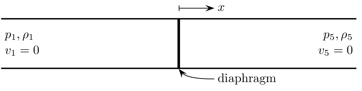
Consider a (one-dimensional) tube filled with two gases that are separated by a
diaphragm. A high-pressure gas is at the left-hand side, and a low-pressure
gas is at the right-hand side. \(p\) denotes the pressure, \(\rho\) the mass
density, \(\gamma\) the ratio of specific heat, and \(v\) the velocity. The gases
are at rest initially (\(t = t_0\) ).
\[
p_1 > p_5 , \quad
\rho_1 > \rho_5, \quad
v_1 = v_5
\]
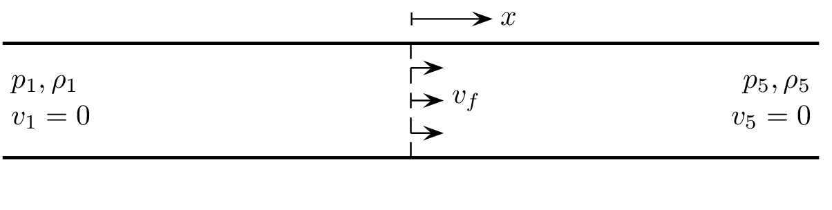
The gas at the high-pressure side is called the driver gas, while the gas at
the low-pressure side is called the driven gas. When the diaphragm is removed,
the driver gas pushes toward the driven gas and the gases around the diaphragm
starts to move to right.
Fig. 14 Gases are at rest in the tube.
Fig. 15 Gases move to right after the diaphragm rupture.
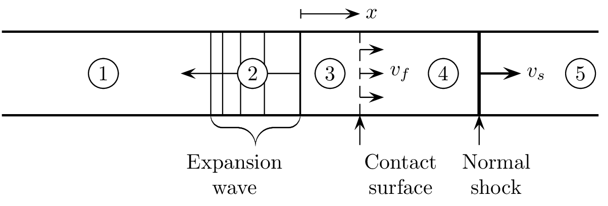
Fig. 16 The zones of flow after the diaphragm disrupts in the tube.
The rupture of the diaphragm generates a right-moving normal shock wave and a
left-moving expansion wave. The flow properties in zones 1 and 5 remain
unchanged. The expansion wave is in zone 2. The contact surface is between
zones 3 and 4. The entropy across the contact surface is discontinuous, but
the condition \(v_3 = v_4 = v_f\) and \(p_3 = p_4\) hold. The right-moving normal
shock wave is between zones 4 and 5. Analytical solution of the problem can be
obtained by solving the problem of the moving shock wave and the expansion wave
[And03 ] .
Moving Normal Shock
Across zones 4 and 5 there is a normal shock moving at the speed \(v_s\) . The
gas velocity \(v_5\) in zone 5 is 0. The conservation of mass, momentum, and
energy across the normal shock moving at the speed \(v_s\) are written as
(48) \[\rho_4 (v_s - v_4) = \rho_5 v_s\]
(49) \[p_4 + \rho_4 (v_s - v_4)^2 = p_5 + \rho_5 v_s^2\]
(50) \[h_4 + \frac{(v_s - v_4)^2}{2} = h_5 + \frac{v_s^2}{2}\]
Obtain the relationship between \(v_s\) and \(v_s-v_4\) by using Eq.
(48) (conservation of mass)
\[
\begin{gathered}
v_s = \frac{\rho_4}{\rho_5}(v_s - v_4), \quad
v_s - v_4 = \frac{\rho_5}{\rho_4}v_s
\end{gathered}
\]
Substitute the equation above to Eq. (49) to have
\[\begin{split}
\begin{gathered}
p_4 - p_5
= \rho_5 v_s^2 \left(1 - \frac{\rho_5}{\rho_4}\right)
\\
\Rightarrow \quad
v_s^2
= \left(\frac{\rho_4}{\rho_5}\right)
\left(\frac{p_4 - p_5}{\rho_4 - \rho_5}\right),
\quad
(v_s - v_4)^2
= \left(\frac{\rho_5}{\rho_4}\right)
\left(\frac{p_4 - p_5}{\rho_4 - \rho_5}\right)
\end{gathered}
\end{split}\]
Recall the relationship \(h = e + \frac{p}{\rho}\) and use the above expressions
of \(v_s^2\) and \((v_s - v_4)^2\) . Substitute them to Eq. (48) to
have
\[
\begin{gathered}
e_4 - e_5 = \frac{p_5}{\rho_5} - \frac{p_4}{\rho_4}
+ \frac{1}{2}
\left(\frac{\rho_4}{\rho_5}
- \frac{\rho_5}{\rho_4}\right)
\left(\frac{p_4 - p_5}{\rho_4 - \rho_5}\right)
\end{gathered}
\]
The Hugoniot equation is obtained for the moving shock
(51) \[e_4 - e_5 = \left(\frac{p_4 + p_5}{2}\right)
\left(\frac{1}{\rho_5} - \frac{1}{\rho_4}\right)\]
By assuming calorically ideal gas, \(e = c_v T\) , \(\gamma = \frac{R}{c_v} + 1\) ,
and \(p = \rho RT\) , the Hugoniot equation leads to
(52) \[\frac{T_4}{T_5} = \frac{p_4}{p_5}
\left(
\frac{\dfrac{\gamma + 1}{\gamma - 1}
+ \dfrac{p_4}{p_5}}
{1 + \dfrac{\gamma + 1}{\gamma - 1}
\dfrac{p_4}{p_5}}
\right)\]
(53) \[\frac{\rho_4}{\rho_5} =
\left(
\frac{1 + \dfrac{\gamma + 1}{\gamma - 1}
\dfrac{p_4}{p_5}}
{\dfrac{\gamma + 1}{\gamma - 1}
+ \dfrac{p_4}{p_5}}
\right)\]
Define the Mach number of the moving normal shock \(M_s = v_s / a_5\) . The
relation of the pressure across the shock wave is
\[
\frac{p_4}{p_5}
= 1 + \frac{2\gamma}{\gamma + 1}(M_s^2 - 1)
\quad \Rightarrow \quad
M_s = \sqrt{
\frac{\gamma + 1}{2\gamma}
\left(\frac{p_4}{p_5} - 1\right) + 1}
\]
Aided by the definition of \(M_s\) , the velocity of the shock can be written as
(54) \[v_s = a_5
\sqrt{\frac{\gamma + 1}{2\gamma}
\left(\frac{p_4}{p_5} - 1\right) + 1}\]
Plug Eq. (53) and Eq. (54) to Eq.
(48) (conservation of mass) to have
\[\begin{split}
\begin{aligned}
v_4 &= \left(1 - \frac{\rho_5}{\rho_4}\right) v_s
\\
&= a_5 \left(1 - \frac{\rho_5}{\rho_4}\right)
\sqrt{\frac{\gamma + 1}{2\gamma}
\left(\frac{p_4}{p_5} - 1\right) + 1}
\\
&=
\frac{a_5}{\gamma}
\left(\frac{p_4}{p_5} - 1\right)
\left[
\left(\frac{\gamma+1}{2\gamma}\right)
\left(\frac{p_4}{p_5} - 1\right) + 1
\right]^{-\frac{1}{2}}
\end{aligned}
\end{split}\]
Further simplify to get
(55) \[v_4 = \frac{a_5}{\gamma}
\left(\frac{p_4}{p_5} - 1\right)
\left(
\dfrac{\dfrac{2\gamma}{\gamma+1}}
{\dfrac{p_4}{p_5}
+ \dfrac{\gamma-1}{\gamma+1}}
\right)^{\frac{1}{2}}\]
The value of the speed of sound (assuming calorically ideal gas) can be
obtained by
\[
a = \sqrt{\gamma R T} = \sqrt{\frac{\gamma p}{\rho}}
\]
Expansion Wave
By using the method of characteristics, the solution of the expansion wave in
zone 2 is obtained. The speed of sound is
(56) \[\frac{a}{a_1}
= 1 - \frac{\gamma - 1}{2}\frac{v}{a_1}\]
Aided by the relation \(a = \sqrt{\gamma R T}\)
(57) \[\frac{T}{T_1} =
\left[1 - \frac{\gamma - 1}{2}
\left(\frac{v}{a_1}\right)\right]^2\]
(58) \[\frac{p}{p_1} =
\left[1 - \frac{\gamma - 1}{2}
\left(\frac{v}{a_1}\right)\right]^{
\frac{2\gamma}{\gamma-1}}\]
(59) \[\frac{\rho}{\rho_1} =
\left[1 - \frac{\gamma - 1}{2}
\left(\frac{v}{a_1}\right)\right]^{
\frac{2}{\gamma-1}}\]
Plugging Eq. (56) into the characteristic (passing
origin)
\[
\frac{\dif x}{\dif t} = v - a
\quad \Rightarrow \quad x = (v - a) t
\]
and obtain
\[
v = \frac{2}{\gamma + 1}\left(a_1 + \frac{x}{t}\right)
\]
The head of the left-running expansion wave moves at \(-a_1\) , the
speed of sound in zone 1.
Connect the Shock Wave and Expansion Wave Solutions
The relationship between the shock wave and expansion wave in the shock tube
can be obtained by the condition across the contact surface, \(v_3 = v_4 = v_f\)
and \(p_3 = p_4\) .
Recall Eq. (55) for the flow speed in zone 4. Recall Eq.
(58) . The flow speed in zone 3 and 4 can be expressed by
using the pressure ratio as
\[
v_3 = \frac{2 a_1}{\gamma - 1}
\left[
1 - \left(\frac{p_3}{p_1}\right)^{\frac{\gamma-1}{2\gamma}}
\right]
\]
Because \(p_3 = p_4\)
(60) \[v_3 = \frac{2 a_1}{\gamma - 1}
\left[
1 - \left(\frac{p_4}{p_1}\right)^{\frac{\gamma-1}{2\gamma}}
\right]\]
Because \(v_3 = v_4\) , by combining Eq. (55) and Eq.
(60) , we have
\[
\frac{a_5}{\gamma}
\left(\frac{p_4}{p_5} - 1\right)
\left(
\dfrac{\dfrac{2\gamma}{\gamma+1}}
{\dfrac{p_4}{p_5}
+ \dfrac{\gamma-1}{\gamma+1}}
\right)^{\frac{1}{2}}
= \frac{2 a_1}{\gamma - 1}
\left[
1 - \left(\frac{p_4}{p_1}\right)^{\frac{\gamma-1}{2\gamma}}
\right]
\]
It can be rearranged to relate \(\frac{p_1}{p_5}\) to \(\frac{p_4}{p_5}\) as
\[
\frac{p_1}{p_5} = \frac{p_4}{p_5}
\left\{
1 - \frac
{(\gamma-1)\dfrac{a_5}{a_1}
\left(\dfrac{p_4}{p_5} - 1\right)}
{\sqrt{2\gamma
\left[
2\gamma
+ (\gamma+1)\left(\dfrac{p_4}{p_5}-1\right)
\right]}}
\right\}^{-\frac{2\gamma}{\gamma-1}}
\]